Disclaimer: All of this is best effort. Feel free to let me know if you spot any mistakes.
Exercise 18.1.
I do not provide solutions for parts (a) and (b). I have calculated answers (c)-(e) by writing this Octave script.
(c) These numbers are obtained by using the definitions (18.3)-(18.5) in [1]:
-
$\kappa(A)=42429.23542$,
-
$\theta=0.68470$,
-
$\mu=1.0$
(d) These condition numbers and upper bounds are obtained by using formulas from Theorem 18.1.:
-
$\kappa_{b \rightarrow y}=1.2910$
-
$\kappa_{b \rightarrow x}=54775.17704$
-
$\kappa_{A \rightarrow y} \leq 54775.17707$
-
$\kappa_{A \rightarrow x} \leq 1469883252.86400$
(e) The perturbation $\delta b$ that causes the relative error of \(y\) to be equal to $\kappa_{b \rightarrow y}$ is any perturbation in the range of $A$. We can get such perturbation by multiplying any vector \(v\) that is not orthogonal to the \(range(A)\) by a projector into the range of $A$: $\delta b=AA^+v$. I used $\delta b=AA^+[1 \; 1 \; 1]'$ and got relative error $err_{b\rightarrow y}=1.2910$. You can find the code for this as for any subsequent calculations for problem 18.1. in this script.
The perturbation $\delta b$ that achieves relative error of x equal to the condition number $\kappa_{b \rightarrow x}$ is one where \(\|A^+\delta b\|_2=\|A^+\|_2\|\delta b\|_2\). We now construct that kind of $\delta b$.
We know that \(\|A^+\|_2=1/\sigma_n\) where \(\sigma_n\) is the n-th and smallest singular value of $A$. We also know that \(A^+=V\Sigma^+U^*\), with \(A=U\Sigma V^*\) being a singular value decomposition of A (see Wikipedia entry on Moore-Penrose pseudoinverse). $\Sigma^+$ is a diagonal matrix with i-ith diagonal entries being $1/\sigma_i$ for non-zero singular values $\sigma_i$ of $A$ and zero elsewhere. In our particular case $n=2$ and $m=3$ so \(\sigma_n=\sigma_2\). If we choose $\delta b=U[0 \; 1 \; 0]’$ we get: \(\begin{eqnarray}\|A^+\delta b\|_2 &=& \|V \Sigma^+U^*U\begin{bmatrix}0 \\ 1 \\ 0\end{bmatrix}\|_2 \nonumber \\ &=&\|\Sigma^+ \begin{bmatrix}0 \\ 1 \\ 0\end{bmatrix}\|_2 \nonumber \\ &=& \frac{1}{\sigma_2}\|\begin{bmatrix}0 \\ 1 \\ 0\end{bmatrix}\|_2 \nonumber \\ &=& \|A^+\|_2\|U \begin{bmatrix}0 \\ 1 \\ 0\end{bmatrix}\|_2 \nonumber \\ &=& \|A^+\|_2\|\delta b\|_2 \end{eqnarray}\)
Above we use the fact that \(\| \cdot \|_2\) norm is unitarily invariant (the norm of the vector does not change when the vector is multiplied by a unitary matrix). The key here was to place a non-zero value only in the n-th (2nd) entry of the vector $U$ is multiplied by. That way we select the \(1/\sigma_n=1/\sigma_2\) value from \(\Sigma^+\).
When using the above described \(\delta b\), I obtained relative error \(err_{b \rightarrow x}=54775.17704\).
While the previous two errors achieved the condition number exactly, the following will not reach the upper bound given in (d), but will come close to it instead.
\(y\) only depends on the $range(A)$. From [1], Tilting the range section we see that the biggest tilt of the $range(A)$ for some fixed value of \(\|\delta A\|_2\) is achieved when \(\delta A=\delta p \cdot v_n\) where $v_n$ is the right singular vector of $A$ associated with its smallest singular value $\sigma_n$ which in the case of this problem is $\sigma_2$. $\delta p$ is a vector orthogonal to the range of $A$. I calculated $\delta p$ as: \(\begin{eqnarray} \nonumber \\ \delta p = (I-AA^+)\begin{bmatrix}1 \\ 1 \\ 0\end{bmatrix}/10^6 \end{eqnarray}\)
And the final perturbation of \(A\) is \(\delta A=\delta p v_2\) where $v_2$ is obtained as the second column of $V$ from $A=U \Sigma V^*$.
The error obtained using this perturbation was $err_{A \rightarrow y}=34639.57287$. The difference between $err_{A \rightarrow y}$ and the uppder bound for $\kappa_{A \rightarrow y}$ can be explained by the relationship between \(y=[2 \; 2.0001 \; 2.0001]'\) and the second left singular vector \(u_2\). Let us look at the two left singular vectors of $A$ that are associated with non-zero singular values: \(\begin{eqnarray}u_1=\begin{bmatrix}-5.77e-01 \\ -5.77e-01 \\ -5.77e-01\end{bmatrix} \\ \nonumber \\ u_2= \begin{bmatrix}8.17e-01 \\ -4.08e-01 \\ -4.08e-01\end{bmatrix}\end{eqnarray}\)
We see that $y$ is approximately aligned with the first left singular vector. This means it is roughly perpendicular to the plane in which the tilt for the described perturbation is made. As explained in [1] this reduces the error by a factor of $\sin \theta$. Indeed we get \(err_{A \rightarrow y} / \sin \theta = 54771.06913\) which is very close to the upper bound we obtained for \(\kappa_{A \rightarrow y}\).
You might ask why not tilt the range in the plane that contains the origin and the points $b$ and $y$ as was done in the section Sensitivity of y to Perturbations in A of [1]. The answer is that due to big difference between $\sigma_1$ and $\sigma_2$, the angle of the tilt of the range while keeping the same \(\|\delta A\|_2\) is much smaller resulting in an error that is significantly less than both the above calculated \(err_{A \rightarrow y}\) and upper bound for \(\kappa_{A \rightarrow y}\).
The bound for the final error \(err_{A \rightarrow x}\) has two terms, one that depends on changes of $A$ that do not alter its range and the other term that is affected by tilting of the range of $A$. The first term is $\kappa(A)$ and the second \(\kappa(A)^2\tan\theta/\mu\). In our example $\mu=1.0$ so the overall error is much more affected by tilting the range than the changes in the mapping of points within the range, since that term contains the quadratic factor $\kappa(A)^2$. Therefore I picked the same perturbation as for \(err_{A \rightarrow y}\) since that is the perturbation that causes the largest tilt of the range of \(A\) for a given \(\|\delta A\|_2\). Thus obtained relative error is \(err_{A \rightarrow x}=1469620366.28139=0.9982 \cdot \text{upper_bound}(\kappa_{A \rightarrow x})\).
Exercise 18.2.
If many variables are used, some of them may be highly correlated. For example, parents’ level of education and parents’ annual income are likely heavily correlated on a large sample of people. This would result in having a very low smallest singular value of \(A\) and a very high \(\kappa(A)\) leading to high condition number $\kappa_{A \rightarrow x}$. This means that a small change in \(A\) can cause a big change in the resulting \(x\). But the point of this problem is to capture trends. So a small change in the input data such as somebody having 1 year of graduate education vs. 2 years with the same annual income or 2 point difference in IQ should not substantially affect the importance the solution assigns to different factors.
Exercise 18.3.
(a) This solution is based on [2].
Let us simplify the problem by assuming that at every point on the water surface we have ripples angled in all direction. Let \(\alpha\) be the maximum angle at which the ripples curve.
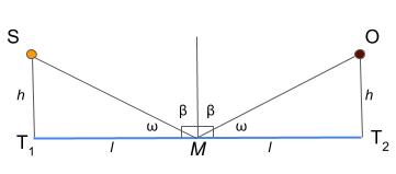
The incoming light ray falls on a surface at some angle $\beta$ to the surface normal and reflects along a line that forms the same angle with the normal but on the other side of it in the plane made by the incoming ray and the normal. See Figure 1. below :

Figure 1.
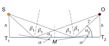
This means that a light ray from the house that falls in the middle of the lake on a piece of water with no ripples will reflect so it falls in the observers eyes, since both the light source and the observer are at the same height. However, if the reflecting surface is at some angle, then the distance between the light source and the reflecting surface needs to be adjusted for the light to reach the observer. This is depicted in Figure 2. below:

Figure 2.
We see from the Figure 2. that if the reflecting surface is angled with the sharper angle turned towards the light source then the reflection point needs to be closer to the light source than the observer if it is to reach the observer. The situation is reversed when the more oblique angle of the reflecting surface is turned to the light source. Also, as visible from the Figure 2. above, tilting the reflecting surface by \(\alpha\) towards the observer and tilting it by \(\alpha\) away from the observer results in two symmetrical cases.
Here we will calculate the ratio of width and length of the vertical streak as perceived by the observer and not the ratio of width and height as they are at the water surface at the points where the light we see is reflected.
We are going to follow the assumption that the perceived dimension of the object is proportional to the angle the endpoints of the object subtend at the eye (See here and here). The perceived dimension of the object is \(n\cdot\gamma\) where \(\gamma\) is the subtended angle and \(n\) is the distance from nodal points to the retina of the eye: something like the diameter of the eyeball.
What limits the length of the vertical streak is the maximum angle \(\alpha\) at which the water ripples (see Figure 2.). We need to calculate the angle \(\gamma\) from Figure 2. because that is the angle that is subtended at the eye of the observer for the length of the vertical streak of light: \(\begin{eqnarray} \alpha_1=\frac{\pi}{2}-\beta_1-\alpha \nonumber \\ \alpha_2=\frac{\pi}{2}+\alpha-\beta_1 \nonumber \\ \label{eq:gamma-1} \alpha_2-\alpha_1=2\alpha \\ \alpha_1+\gamma+\pi-\alpha_2=\pi \nonumber \\ \label{eq:gamma-2} \gamma=\alpha_2-\alpha_1 \\ \gamma=2\alpha \end{eqnarray}\)
Using \eqref{eq:gamma-1} and \eqref{eq:gamma-2} we arrived at the angle \(\gamma=2\alpha\) as the angle subtending the length of the light streak at the observer’s eye.
Width of the streak varies at different points. We will use the point in the middle of the lake for our calculations. The actual width on the lake in the middle is the biggest width the streak attains on the lake. However, according to [2] that is not the point of the maximum perceived length. Nevertheless, that is the point they use to caculate the width and so will I, because the calculations are easy. Besides, the width of the streak varies anyways.

Figure 3.
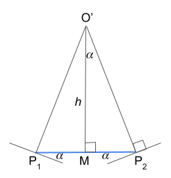
In the middle of the lake, even at some point away from the plane \(SOT_2\), the light ray has an equidistant path from the source to that point and from that point to the observer. The reflecting surface at the point must be inclined in order to account for the needed change in the direction of the travel. The reflecting surface is rotated around the axis that is parallel to the segment \(T_1T_2\) (Figure 2.) and passes through the point of reflection. In the Figure 3. we show the inclination of the reflecting surface which is symmetric on the two sides and an observer (or light source) projected onto a plane perpendicular to \(T_1T_2\) passing through point \(M\) in the middle of the lake (see Figure 2. for point locations). The two sides of the depicted triangle \(P_1O'\) and \(P_2O'\) are positioned on the normals to the reflecting planes. \(P_1\) and \(P_2\) are points of the light reflection. From the image we see that the angles \(\angle P_1O'M=\angle MO'P_2=\alpha\). Therefore the actual width of the streak on the lake is \(2 h\tan \alpha\).
The angle subtended at the eye for the width of the streak is \(\angle P_1OP_2=\delta\). We know that the length \(\overline{MO}=\sqrt{h^2+l^2}\) with \(h=50m\) and \(2l=1000m\). By using the calculated streak width we get \(\tan (\delta/2)=h \tan \alpha/\sqrt{h^2+l^2}\). We know that value of small angles in radians is nearly equal to their tangens. In our case we have \(\frac{h}{\sqrt(h^2+l^2)}\approx 0.01\) which means that \(\tan (\delta/2)\) is small for at least \(\alpha \leq 45^\circ\). [2] makes the assumption that in normal weather circumstances \(\alpha\approx 15^\circ\). Taking that into account we can write: \(\begin{eqnarray} \nonumber \\ \delta \approx \frac{2h\tan\alpha}{\sqrt{h^2+l^2}} \end{eqnarray}\)
And finally, the ratio of the perceived width and length, with assumed \(\alpha=15^\circ\), is \(r=\frac{\delta}{\gamma}=h\tan\alpha/(\alpha\sqrt{h^2+l^2})=0.1018\). For small \(\alpha\) we have \(\tan\alpha \approx \alpha\) so we can write \(r\approx\frac{h}{\sqrt(h^2+l^2)}=\sin \omega=0.0995\). We see that for \(\alpha=15^\circ\) the two calculations are quite close.
(b) This problem is related to the way \(\|\delta y\|_2\) behaves when we tilt the range of \(A\) by a fixed \(\delta \alpha\) in different planes/around different axes. When the range is tilted in the plane \(0-b-y\), \(\|\delta y\|_2\) attains its maximum. If the range is tilted in the plane passing through \(b\) and \(y\) that is perpendicular to segment \(0-y\), \(\|\delta y\|_2\) attains its minimum value that is smaller than its maximum by a factor of \(\sin \theta\). Similarly, in this problem we get different values for the width and the length of the vertical streak with the maximum length achieved by tilting the reflecting surface in the plane \(SOT_2\) i.e. around rotational axes perpendicular to that plane. If we tilt the reflecting plane around other axes at other points in the lake, the dimension of the streak shortens. We can see that particularly when we observe the width of the light streak in the middle of the lake as we did in part (a) of the problem. The approximate ratio of the width and the length has a similar formulation to the ratio of maximum and minimum \(\|\delta y\|_2\) for a fixed \(\delta \alpha\): \(\sin\omega\) with \(\omega\) in the case of this problem being the angle \(\angle OMT_2\), i.e. the angle between the line connecting the observer and the middle point of the lake on the plane perpendicular to the lake containing the observer and the source and the horizontal line on the lake passing through that plane.
Exercise 18.4.
The condition number of $y$ becomes $0$ with respect to perturbations of $A_{mxn}$ when $m=n$ because an assumption was made that $A$ has full rank. Since $m=n$ that means that $A$ is non-singular. We know that for small enough perturbations $E$ of a non-singular $A$, $B=A+E$ is non-singular (for the proof see Theorem 3 in this write-up). Condition number is defined in the limit for small perturbations, so we may assume that the perturbed $B$ is non-singular and full rank, much like $A$. Since both $A$ and be $B$ are square matrices of full rank and same dimensions, their ranges are the same. We know that $y$ is a projection of $b$ into the range of $A$. With perturbations it becomes a projection of $b$ into the range of $B$. Since the two ranges are the same, the projection remains the same across different perturbations. Therefore, the condition number for $y$ with respect to perturbations in $A$ becomes $0$ when $m=n$.
References
[1] Trefethen, L., and Bau, D. Numerical Linear Algebra, SIAM, (1997).
[2] Minnaert, M. The Nature of Light and Color in the Open Air, Dover Publications Inc., (1954)